The Seismo-Electric Geophysical Method

1. Introduction

The seismo-electric effect refers to the generation of electrical fields as a result of seismic wave propagation through fluid-saturated porous media. This phenomenon provides a powerful tool for subsurface exploration, integrating seismic and electromagnetic methods to reveal information about porosity, permeability, and fluid content. This paper delves into the theoretical foundations, historical development, and various geophysical applications of the seismo-electric method. Detailed discussions on key concepts such as the electric double layer, zeta potential, and electrokinetic coupling are provided, along with a thorough examination of the rise time interpretation, seismic sources, data collection methods, and the limitations and assumptions of the seismo-electric method.

2. Background

The theory of electro-seismic phenomena began with Frenkel (1944), who postulated equations describing fluid-solid flow induced by seismic waves using the Helmholtz-Smoluchowski equation. This equation only accounted for co-seismic electric fields and did not include electromagnetic wave generation at interfaces. Biot's theory (1956, 1962) further developed the field by describing seismic wave propagation in fluid-saturated porous media, introducing the concept of slow and fast pressure waves, with slow waves being dissipative and regenerated at interfaces. Nourbehecht (1963) explored electrokinetic coupling but did not use Biot's theory and overlooked shear wave contributions to electro-seismic conversion.

Later developments included Neev and Yeatts (1989), who attempted to model mechanical and electric field coupling but did not use the full set of Maxwell's equations, incorrectly concluding that shear waves do not generate electromagnetic waves. Pride (1994) advanced the theory by incorporating Maxwell's equations and deriving macroscopic governing equations for electro-seismic phenomena, showing that no net electrical current exists within seismic waves, thus no electromagnetic radiation is produced.

Haartsen (1995) and Pride and Haartsen (1996) demonstrated that plane waves in homogeneous porous media do not generate electromagnetic waves. However, at interfaces between media with different electro-seismic properties, an imbalance in streaming current density generates independent electromagnetic waves, an effect observed in various field studies. Haartsen and Pride (1997) confirmed that interface responses resemble those of an oscillating electric dipole at the interface. Subsequent research by Haartsen et al. (1998), Ranada Shaw et al. (2000), and Garambois and Dietrich (2001) further investigated the effects of porosity, permeability, and salinity on electro-seismic responses and derived transfer functions linking seismic wave-induced displacements to co-seismic electric and magnetic fields, validated against field data.

3.The seismo-electric effect

The seismo-electric effect can be observed when a fast-traveling p wave intersects a water saturated interface of differing anelastic or electrical properties (Pride 1994). The seismo-electric effect is in effect a form of converted energy which is released as dissipated energy. This conversion of energy takes place when a fast-moving P-wave produces slower P waves as it passes through the interface. These slow P waves produce much more movement between the rock and water. This in turn leads to a high loss of energy in the form of heat due to friction and seismo-electric effects, such as electromagnetic radiation due to ionic movement. seismo-electric signals are produced by the out of phase motion between all the ions in the water and those attached to the rock. The relationship between applied pressure P and electric potential response  for a porous rock is generally given by the following equation (Millar and Clarke 1997):

f  = electrical potential response or streaming potential

C = electrokinetic coefficient

P = applied pressure

ee₀ = permittivity of the pore space

z = zeta potential

h = fluid viscosity

s = electrical conductivity

This equation relates the electrical potential response f developed in a porous rock to the stimulus of an incident pressure change P, allowing the rock to be characterized by C on a macroscopic scale when modelling such electrokinetic responses.

4. Seismo-electric points of difference

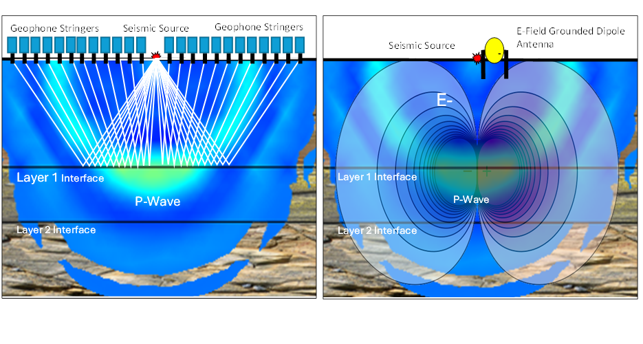
Reflection Seismology:

• Requires many geophone sensors connected in strings over vast distances

• Geophone line strings often require bush and fence clearing for accessibility

• Collects lateral data and builds vertical information.

• Is labour intensive and time consuming.

• Is designed to collect data over wide areas, not practical for small projects.

• Is subject to two-way travel seismic attenuation

• Only geological mechanical data is collected

Electro-seismic:

• Requires only one grounded dipole antenna

• Does not require any clearance or defencing.

• Collects vertical and lateral data.

• Is not labour intensive or time consuming

• Designed for small or large area surveys.

• Is only subject to one-way seismic attenuation.

• Geological mechanical and electrical data is collected

5. Governing Equations

A full set of governing equations is provided by Pride (Pride, 1994) that describe the coupling of seismic and electromagnetic fields in the time domain, using volume averaging arguments.

Discussed here are a full set of equations governing the seismo-electric conversions, as described by (Pride, 1994). These equations collectively describe the complex interactions between seismic waves, electric fields, magnetic fields, and fluid flow in the Earth's subsurface. By using these equations, geophysicists can extract valuable information about the physical properties of subsurface formations, such as their composition, porosity, permeability, fluid content, and mechanical properties. This information is essential for exploring and managing natural resources like oil, gas, and groundwater, as well as for understanding geological processes.

Momentum balance equation

In seismo-electric coupling, seismic waves (mechanical energy) can generate electromagnetic fields when they pass through a fluid-saturated porous medium. This is due to the relative motion between the solid matrix and the pore fluid, which causes an electrokinetic effect—specifically, the movement of charged particles within the fluid relative to the solid matrix generates an electric field.

This equation (Pride, 1994) describes the momentum balance in such a medium, where the mechanical stress (related to seismic waves) is balanced by inertial forces due to both the solid matrix and the pore fluid, with the latter contributing to the generation of electromagnetic signals.

Ñ· t = Ρu˙˙ + Ρ f w˙˙

• : This term represents the divergence of the stress tensor (), which is related to the mechanical stress within the material. In a seismo-electric context, this stress is induced by seismic waves traveling through the Earth.
• : This is the mass density of the medium, representing the material's density where the seismic waves are propagating.
• : This represents the acceleration of the solid matrix of the material due to seismic waves. The term  corresponds to the inertial forces resulting from the acceleration of the medium’s solid matrix.
• : This is a coupling factor that accounts for the interaction between the seismic waves and the electromagnetic fields. In seismoelectric phenomena, seismic waves can generate electric fields in a porous medium where the pore fluid contains ions.
• : This represents the acceleration of the pore fluid relative to the solid matrix. The term  represents the contribution of the pore fluid's motion to the overall force balance, which is important in the generation of seismo-electric signals.

In summary, this equation in the context of seismo-electric phenomena describes how seismic waves propagating through a porous medium with fluid-filled pores can induce electromagnetic fields through the interaction of the solid and fluid components of the medium. This is a key aspect of understanding how seismic waves can be detected via their associated electric fields, a process used in seismo-electric surveys for subsurface exploration.

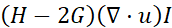
Stress-strain relationship equation

This equation (Pride, 1994) describes the stress tensor  in a poroelastic medium, incorporating the effects of both mechanical deformations of the solid matrix and the fluid movement within the pores. In the context of seismo-electrics, this equation plays a crucial role in understanding how mechanical stress in a porous medium can lead to electric fields and currents.

• : The stress tensor, which represents the internal forces (stresses) within the material in response to deformation.
• : This is a material parameter related to the bulk modulus of the solid matrix, which quantifies the material's resistance to uniform compression.
• : This represents the shear modulus, also known as the modulus of rigidity, which describes the material's response to shear deformations (i.e., changes in shape without a change in volume).
• : The divergence of the displacement vector , representing the volumetric strain, or the relative change in volume of the solid matrix due to deformation.
• : The identity tensor, which, when multiplied by a scalar, gives a tensor proportional to the identity matrix, indicating isotropic stress (equal stress in all directions).
• : This term represents the symmetric part of the displacement gradient tensor, describing the strain in the solid matrix due to deformation. The transpose  accounts for the symmetry of the stress tensor.
• : This is a coupling parameter related to the interaction between the pore fluid pressure and the solid matrix stress.
• : The divergence of the relative displacement vector  of the fluid within the pores, which represents the change in fluid content or fluid pressure within the porous medium.

Interpretation in Seismo-electric Terms:

1. First Term: :

• This term represents the isotropic stress in the solid matrix due to changes in volume (volumetric strain) of the solid matrix. In a seismo-electric context, this could relate to how seismic compressional waves (P-waves) induce stress in the porous medium.

2. Second Term: :

• This term accounts for the deviatoric (shear) stress in the solid matrix. Shear stresses are crucial in describing the response of the medium to shear waves (S-waves), and in seismo-electrics, this can be linked to the generation of electric fields due to the shear deformation of the matrix.

3. Third Term: :

• This term introduces the effect of pore fluid pressure on the stress within the solid matrix. In seismo-electric phenomena, this is important because changes in pore fluid pressure due to seismic waves can generate electric potentials via electrokinetic effects, such as streaming potentials.

Seismo-electric Implications:

• The equation combines the mechanical deformation of the solid matrix and the influence of the pore fluid, capturing the poroelastic behavior of the medium.
• The stress tensor  includes contributions from both the solid matrix deformation and the fluid movement within the pores. In a seismoelectric context, this is critical because the interaction between seismic waves and the fluid-saturated porous medium can lead to the generation of electric fields (seismoelectric signals).
• The coupling parameter  reflects how fluid pressure changes contribute to the overall stress, which is a key factor in generating the seismoelectric response observed in subsurface exploration.

In summary, this equation provides a detailed description of how stress is distributed in a porous medium under the influence of both seismic waves and fluid movement. This stress distribution is directly related to the generation of seismo-electric signals, which are used to detect and map subsurface features such as fluid reservoirs or fractures.

Biot's effective stress equation

This equation (Pride,1994) describes the relationship between pore pressure , the volumetric strain of the solid matrix, and the fluid content in a poroelastic medium. This equation is significant in the context of seismo-electrics, as it links mechanical deformation to fluid pressure changes, which are key to the generation of seismoelectric signals.

• : This represents the pore pressure, which is the pressure of the fluid within the pores of the porous medium. In seismoelectrics, changes in pore pressure can induce electric fields due to electrokinetic effects.
• : This is a poroelastic coupling coefficient, which represents how changes in the volumetric strain of the solid matrix affect the pore pressure. It reflects the interaction between the solid matrix deformation and the fluid pressure.
• : The divergence of the displacement vector , representing the volumetric strain of the solid matrix (i.e., the relative change in volume due to deformation). When a seismic wave passes through a porous medium, it causes the solid matrix to deform, which in turn affects the pore pressure.
• : This is the fluid modulus, representing how changes in the fluid content or fluid pressure relate to changes in the overall stress and pore pressure. It is a measure of the fluid's compressibility within the pores.
• : The divergence of the fluid displacement vector , representing the change in fluid content or fluid flow within the pores. This term describes how fluid movement affects the pore pressure.

In the context of seismo-electrics, this equation has the following implications:

Pore Pressure Generation:

o The equation describes how the pore pressure  is generated in response to mechanical deformations (volumetric strain of the solid matrix, ) and changes in fluid content (represented by ).

o When a seismic wave (such as a P-wave) travels through a fluid-saturated porous medium, it causes the solid matrix to compress and expand (), which in turn changes the pore pressure. Similarly, the relative motion of the pore fluid () also affects the pore pressure.

Seismo-electric Signal Generation:

o In seismo-electric phenomena, changes in pore pressure can induce electric fields through electrokinetic effects, such as the streaming potential. The streaming potential arises when the pore fluid moves relative to the solid matrix, dragging ions in the fluid and generating an electric field.

o The term  indicates that the volumetric strain of the solid matrix contributes to pore pressure changes, while  indicates the contribution of fluid movement.

Poroelastic Response:

o This equation is part of the poroelastic theory, specifically describing the coupling between mechanical stress, pore pressure, and fluid flow. In seismo-electrics, understanding this relationship is crucial for interpreting how seismic waves can generate electromagnetic fields in the Earth's subsurface.

This equation is a constitutive relation within the framework of Biot's theory of poroelasticity, specifically describing the generation of pore pressure in response to mechanical deformation of the solid matrix and changes in fluid content. In seismo-electrics, this relationship is key to understanding how seismic waves induce pore pressure changes, which in turn can generate electric fields through electrokinetic effects, enabling the detection of seismo-electric signals.

Fluid flow equation

This equation (Pride,1994) can be interpreted in the context of seismo-electrics as describing the movement of the pore fluid () within a porous medium under the influence of various forces, including electric fields, pressure gradients, and mechanical accelerations.

• : This represents the velocity of the pore fluid within the porous medium, or the rate of change of the fluid displacement vector . It describes how the fluid within the pores of a solid matrix moves.
• :

o Here,  is a coupling coefficient that relates the electric field  to the fluid flow.

o The term  represents the electrokinetic flow of the fluid induced by the electric field. This is related to the electrokinetic phenomena where an applied electric field can cause fluid movement in the pores due to the interaction with the charged fluid particles.

• :

o  is the permeability of the medium, which measures the ease with which fluid can flow through the pores.

o  is the pressure gradient driving the fluid flow. The term  represents Darcy's law, which states that the fluid velocity is proportional to the pressure gradient. This term describes how fluid moves from high-pressure regions to low-pressure regions within the porous medium.

• :

o  is the density of the fluid,  is a coupling coefficient related to the dynamic viscosity or inertial effects, and  represents the interaction factor between the solid and fluid phases.

o  is the acceleration of the solid matrix. The term  represents the inertial forces acting on the fluid due to the acceleration of the solid matrix. In seismoelectrics, when seismic waves propagate through the porous medium, they cause the solid matrix to accelerate, which in turn affects the movement of the fluid within the pores.

Interpretation in Seismo-electric Context:

Electrokinetic Flow ():

o This term highlights the electrokinetic effects where the presence of an electric field can drive the movement of the pore fluid. In seismo-electrics, when seismic waves interact with the subsurface, they can generate electric fields, which in turn can influence the movement of fluids in porous media.

Pressure-Driven Flow ():

o This term describes the classic fluid flow driven by pressure differences within the porous medium, following Darcy's law. In the context of seismo-electrics, seismic waves can create pressure gradients that drive fluid movement, which can then interact with the electric fields generated by the waves.

Inertial Forces ():

o This term accounts for the inertial effects on the fluid caused by the acceleration of the solid matrix. As seismic waves propagate, they cause the solid matrix to move, which induces corresponding movements in the pore fluid due to inertia. This interaction is crucial for understanding how seismic waves can influence fluid dynamics in the subsurface.

In summary, this equation describes the velocity of the pore fluid in response to multiple driving forces: an electric field, a pressure gradient, and the inertial effects from the solid matrix's acceleration. In seismo-electric phenomena, these factors are all interconnected. Seismic waves can induce both mechanical and electromagnetic fields, which then interact with the fluid in the pores, potentially leading to observable seismo-electric signals. This equation captures the complex dynamics of fluid flow in a porous medium under the influence of seismo-electric effects.

Seismo-electric current density equation

This equation (Pride,1994) describes the current density  in a porous medium as a result of both electric and mechanical influences. This equation is particularly relevant in the context of seismo-electrics, where seismic waves can generate electric fields and currents in the subsurface.

• : The current density, which represents the electric current per unit area flowing through the porous medium. In seismoelectrics, this is the electric response generated by the coupling of seismic and electromagnetic fields.
• : The electrical conductivity of the medium, a measure of how easily electric charges can move through the material.
• : The electric field, which drives the movement of electric charges, contributing to the current density .
• : A coupling coefficient related to the electrokinetic coupling between the mechanical and electric fields in the medium. This coefficient determines how the pressure gradient and inertial effects translate into electrical current.
• : The gradient of the pore pressure . This term represents how changes in pressure within the fluid-saturated pores drive fluid movement, which can induce an electric current via electrokinetic effects.
• : The density of the fluid within the pores.
• : A coupling factor between the solid matrix and the fluid.
• : The acceleration of the solid matrix due to seismic waves. This term represents the inertial forces acting on the fluid and solid matrix, which can contribute to the generation of an electric current.

Interpretation in Seismo-electric Context:

Ohm's Law Contribution ():

o This term represents the current density generated directly by the electric field  in the medium, following Ohm's law. In seismoelectrics, this can be the primary electric response due to existing electric fields in the subsurface.

Electrokinetic and Inertial Contributions ():

o The term  represents additional contributions to the current density arising from pressure gradients and the inertial effects of seismic waves.

o : This term reflects the electrokinetic effects, where pressure gradients (often caused by seismic waves compressing the medium) can drive fluid movement. This fluid movement, in turn, can induce an electric current (streaming current) due to the relative motion of charged particles within the fluid.

o : This part accounts for the contribution of the inertial forces due to the acceleration of the solid matrix caused by seismic waves. The coupling between these inertial effects and the fluid flow can generate additional current in the medium.

o

Seismo-electric Implications:

In the context of seismo-electrics, this equation describes how seismic waves propagating through a porous, fluid-saturated medium can induce an electric current. The total current density  is a result of:

· Direct electric field effects: As captured by the  term, where the electric field in the subsurface drives the current.

· Electrokinetic effects: The term  represents current generated by fluid flow caused by pressure gradients.

· Inertial effects: The term  reflects the contribution of seismic wave-induced accelerations to the electric current.

This equation is key in understanding how mechanical disturbances (seismic waves) in the Earth's subsurface can be converted into measurable electrical signals, which is the basis for seismo-electric exploration techniques.

This equation is a current density equation in the context of seismo-electrics. It describes how electric currents in the Earth's subsurface are generated by both the electric field and the coupled effects of seismic waves, which induce pressure gradients and accelerations in the porous medium. This coupling between seismic and electromagnetic phenomena is fundamental to the study of seismo-electrics.

Faraday's Law of Induction

This equation (Pride,1994) is one of Maxwell's equations, specifically Faraday's Law of Induction. In the context of seismo-electrics, this equation describes how a time-varying magnetic field  generates an electric field . Here's how it relates to seismoelectrics:

• : The curl of the electric field  represents the tendency of the electric field to circulate around a point. In physical terms, it measures the rotational effect of the electric field in space.
• : This term represents the time rate of change of the magnetic field . According to Faraday's Law, a changing magnetic field induces a circulating electric field.

Interpretation in Seismo-electric Context:

In seismo-electrics, seismic waves propagating through the Earth's subsurface can induce electromagnetic fields due to the motion of charges within fluid-saturated porous media. Here's how the equation plays a role:

Induced Electric Fields:

o As seismic waves travel through a porous medium, they can generate time-varying magnetic fields. According to this equation, these changing magnetic fields then induce electric fields in the surrounding material.

o This is crucial in seismo-electric phenomena because the induced electric fields are part of the signals that can be measured at the surface to gain insights into the subsurface structures.

Coupling of Seismic and Electromagnetic Fields:

o The seismic wave's mechanical energy is partly converted into electromagnetic energy via electrokinetic effects (such as the motion of ions in the pore fluid) and through direct induction processes described by Faraday's Law.

o The equation indicates that the induced electric field is directly related to the rate at which the magnetic field changes, which can be caused by the movement of conducting materials in the Earth's subsurface in response to seismic waves.

Seismo-electric Signal Detection:

o The electric fields generated according to this equation contribute to the seismo-electric signals that are detected by instruments on the Earth's surface. These signals are used to infer properties of the subsurface, such as porosity, fluid content, and the presence of geological features like faults or fractures.

In the context of seismo-electrics, the equation  describes how the time-varying magnetic fields generated by seismic wave-induced movements in the Earth's subsurface induce circulating electric fields. This process is central to the generation of seismoelectric signals, which combine information about both the mechanical and electromagnetic properties of the subsurface. Faraday's Law thus plays a critical role in understanding how seismic energy can be converted into measurable electromagnetic signals.

Ampère's Law with Maxwell's Correction

This equation (Pride,1994) is another of Maxwell's equations, specifically Ampère's Law with Maxwell's correction. In the context of seismo-electrics, this equation describes how magnetic fields () are generated by both electric currents () and the time-varying electric displacement field:

• : The curl of the magnetic field  represents the tendency of the magnetic field to circulate around a point. This term essentially measures the rotational effect of the magnetic field in space.
• : The current density, which is the flow of electric charge per unit area. In seismoelectrics, this can be the current generated by the movement of fluid in a porous medium, driven by seismic waves and electrokinetic effects.
• : The time rate of change of the electric displacement field . The displacement field  is related to the electric field  and the material's properties, and its time derivative represents how changes in the electric field contribute to the magnetic field.

Interpretation in Seismo-electric Context:

In the context of seismo-electrics, this equation describes the generation of magnetic fields due to both electric currents and the changing electric fields that arise from seismic activity in the Earth's subsurface. Here's how it applies:

Generation of Magnetic Fields:

o As seismic waves propagate through the Earth's subsurface, they can induce electric currents () due to electrokinetic effects, such as the movement of ions in the pore fluids.

o These currents generate magnetic fields, as described by the  term in this equation.

Displacement Current Contribution:

o The term  represents the displacement current, which is a concept introduced by Maxwell to account for situations where the electric field changes over time, even in the absence of a physical current.

o In seismo-electrics, the displacement current could be generated by the time-varying electric fields associated with seismic waves, further contributing to the magnetic fields in the subsurface.

Seismo-electric Signal Detection:

o The magnetic fields generated by the combined effects of electric currents and displacement currents are part of the seismo-electric signals that can be detected at the Earth's surface.

o These signals provide information about the subsurface properties, such as the distribution of fluids, the nature of the porous medium, and the presence of geological structures.

In the context of seismo-electrics, the equation  (Ampère's Law with Maxwell's correction) describes how magnetic fields in the Earth's subsurface are generated by both electric currents, which can arise from the movement of fluid in response to seismic waves, and by time-varying electric fields. This equation is crucial for understanding the generation of seismo-electric signals, which are used to explore and map subsurface structures by detecting the electromagnetic fields induced by seismic activity.

Electric displacement equation

This equation (Pride, 1994) is known as the constitutive relation between the electric displacement field  and the electric field , where  represents the permittivity of the material. In the context of seismo-electrics, this equation describes how the material in the Earth's subsurface responds to an electric field.

• : The electric displacement field, which accounts for the effect of free charges and bound charges (those associated with the atoms and molecules of the material) in the presence of an electric field. In seismoelectrics,  represents how the material's internal electric field is affected by external forces, such as seismic waves.
• : The permittivity of the material, which measures how easily a material can become polarized by an electric field. In the Earth's subsurface,  depends on the type of rock or soil and the fluids present in the pores. The permittivity can vary depending on whether the medium is dry, water-saturated, or oil-saturated.
• : The electric field, which is a force field that acts on charges, causing them to move. In seismoelectrics, the electric field can be generated by various processes, including the motion of seismic waves through the subsurface, which can induce charge separation and thus an electric field.

Interpretation in Seismo-electric Context:

In seismo-electrics, this equation is important for understanding how electric fields are influenced by the properties of the Earth's subsurface. Here's how it applies:

Polarization of the Subsurface:

o The electric displacement field  includes both the free charge contributions and the bound charges that are induced by the electric field .

o In the context of seismo-electrics, when seismic waves propagate through a porous medium, they can cause relative motion between the solid matrix and the pore fluids. This motion can lead to charge separation (due to the movement of ions in the fluid), generating an electric field.

Material Response to Electric Fields:

o The permittivity  characterizes how the subsurface material responds to the induced electric field. Different materials (e.g., rocks, water, oil) have different permittivities, which affects the strength of the displacement field .

o This is crucial for seismo-electric exploration, as variations in permittivity can indicate different subsurface materials and fluid content, providing valuable information about the geological structure.

Seismo-electric Signal Generation:

o The equation  helps explain the generation of seismoelectric signals. As seismic waves travel through the Earth's subsurface, they can induce electric fields that polarize the material, creating an electric displacement field .

o The characteristics of the seismo-electric signals (e.g., amplitude, frequency) are influenced by the permittivity of the subsurface materials, which can be used to infer properties like porosity, fluid content, and the presence of different layers or faults.

In the context of seismo-electrics, the equation  describes how the electric displacement field  in the Earth's subsurface is related to the electric field  and the material's permittivity . This relationship is key to understanding how seismic waves induce electric fields and how these fields interact with the subsurface materials to produce seismoelectric signals that can be detected and analyzed for subsurface exploration.

Magnetic constitutive equation

This equation (Pride,1994) is another constitutive relation in electromagnetism, relating the magnetic flux density  to the magnetic field strength , where  is the magnetic permeability of the material. In the context of seismo-electrics, this equation describes how the Earth's subsurface materials respond to magnetic fields, particularly those generated by seismic activity.

• : The magnetic flux density (or magnetic induction), which represents the density of magnetic field lines in a material. It indicates how much magnetic field is produced in a medium in response to a magnetic field strength .
• : The magnetic permeability of the material, which is a measure of how easily a material can support the formation of a magnetic field within itself. In the Earth's subsurface,  varies depending on the type of material, such as rock, water, or other minerals.
• : The magnetic field strength, which represents the magnetic field generated by a current or a changing electric field. In seismoelectrics,  can be induced by the movement of charges due to seismic waves.

Interpretation in Seismo-electric Context:

In seismo-electrics, this equation is crucial for understanding the interaction between magnetic fields and the materials in the Earth's subsurface. Here's how it applies:

Magnetic Field Response in Subsurface Materials:

o The equation  indicates that the magnetic flux density  is directly proportional to the magnetic field strength , with the proportionality constant being the permeability .

o Different subsurface materials have different permeabilities, which means that for the same magnetic field strength , the resulting magnetic flux density  will vary depending on the material.

Magnetic Field Generation by Seismic Waves:

o As seismic waves propagate through the Earth's subsurface, they can cause the movement of charged particles, which generates electric currents (). According to Ampère's Law, these currents generate magnetic fields ().

o The equation  then describes how these magnetic fields are influenced by the permeability of the subsurface materials, determining the resulting magnetic flux density .

Seismo-electric Signal Detection:

o Seismo-electric methods detect electromagnetic signals, including those related to magnetic fields, generated by seismic activity. The relationship  helps in understanding the magnetic component of these signals.

o Variations in the magnetic flux density  detected at the surface can provide information about the subsurface materials, such as their composition and magnetic properties, which are useful for geological exploration.

In the context of seismo-electrics, the equation  describes how the magnetic flux density  in the Earth's subsurface is related to the magnetic field strength  and the material's magnetic permeability . This relationship is key to understanding how magnetic fields generated by seismic-induced currents interact with different subsurface materials, contributing to the seismoelectric signals that are measured and analyzed in subsurface exploration.

6. Electric Double Layer

These equations (Fourie, 2003), (Tuman ,1963), (Shaw ,1969), (Ishido ,1981) and (Pride and Morgan ,1991) describe the distribution of ions within the electric double layer (EDL) in a fluid-saturated porous medium, specifically in the context of the seismo-electric method. The electric double layer, which forms at the interface between a solid surface (such as a mineral grain) and the surrounding pore fluid, is crucial for understanding how seismic waves can generate electrical signals.

The Equations:

Positive Ion Distribution:

This equation describes the concentration  of positive ions at a position  within the electric double layer, influenced by the local electric potential .

Negative Ion Distribution:

This equation describes the concentration  of negative ions at a position  within the electric double layer, influenced by the local electric potential .

Electric Potential Distribution:

This equation describes the electric potential  at a distance  from the solid surface, where  is the potential at the surface and  is the characteristic decay length.

Terms Explained:

· : The concentration of ions (positive or negative) at position  within the electric double layer.

· : The reference concentration of ions when the potential  is zero.

· : The valence of the ion (e.g.,  for a singly charged ion).

· : The elementary charge, representing the charge of a single proton.

· : The electric potential at position  within the electric double layer.

· : Boltzmann's constant, relating temperature to energy.

· : The absolute temperature.

· : The electric potential at the surface of the solid.

· : The characteristic decay length, which describes how quickly the potential decreases with distance from the solid surface.

The EDL is a critical concept in seismo-electrics, as it governs the behavior of ions at the interface between solid surfaces and fluids, influencing how seismic waves generate electrical signals. The EDL is composed of two main parts:

Stern Layer:

· Location and Characteristics: The Stern layer is the inner part of the electric double layer, closest to the solid surface. In this layer, ions are tightly bound to the surface due to strong electrostatic forces.

· Ion Distribution: The ion distribution in the Stern layer does not follow the simple Boltzmann distribution given by the provided equations. Instead, the ions in this layer are more or less fixed in position due to the strong attraction to the surface, resulting in a compact layer where the electric potential  is high but decreases sharply with distance from the surface.

· Relevance to Seismo-electrics: The Stern layer is important in establishing the initial conditions for the potential  that influences the distribution of ions in the Gouy layer. However, because the ions in the Stern layer are relatively immobile, their direct contribution to the seismoelectric signal is limited.

Gouy-Chapman (Diffuse) Layer:

· Location and Characteristics: The Gouy-Chapman layer, or diffuse layer, lies outside the Stern layer and extends further into the fluid. In this layer, ions are less tightly bound and can move more freely, responding to thermal motion and the electric potential.

· Ion Distribution: The equations you provided describe the ion distribution in the Gouy-Chapman layer. Here, the ion concentrations are determined by the balance between the thermal energy (which tends to spread ions out) and the electric potential  (which attracts or repels ions depending on their charge). The exponential terms indicate how the concentration of positive and negative ions decreases or increases with distance from the surface, depending on the sign and magnitude of the potential .

· Electric Potential: The potential  within the Gouy layer decays exponentially with distance from the surface, as described by the equation . This decay length  depends on factors such as the ionic strength of the fluid and the temperature.

· Relevance to Seismo-electrics: The Gouy layer is critical in generating seismo-electric signals. When seismic waves pass through the porous medium, they cause the fluid (and the ions within it) to move relative to the solid matrix. This movement disturbs the ion distribution in the Gouy layer, generating an electric field as the ions are displaced. The resulting electric field can be detected at the surface as part of a seismo-electric signal, providing information about the subsurface properties.

·

Seismo-electric Signal Generation:

· Streaming Potential: In seismo-electrics, when seismic waves induce fluid flow through a porous medium, the ions in the Gouy layer are dragged along with the fluid. This movement creates a streaming potential, a key component of the seismo-electric signal. The magnitude and characteristics of this potential are influenced by the ion distribution described by the equations.

· Ion Redistribution: The redistribution of ions in the Gouy layer due to seismic activity changes the local electric potential , which can lead to the generation of time-varying electric fields detectable as seismoelectric signals.

The equations describe how ions are distributed within the Gouy-Chapman layer of the electric double layer in response to an electric potential . The Stern layer, which is closer to the solid surface, holds more tightly bound ions, while the Gouy layer contains more mobile ions whose distribution is described by these equations. In the seismo-electric method, seismic waves disturb the ion distribution in the Gouy layer, leading to the generation of electrical signals. These signals provide valuable information about subsurface properties such as porosity, permeability, and fluid content, making the understanding of the EDL crucial for interpreting seismo-electric data.

7. Zeta Potential

This equation (Wang, Hu, Guan, 2015) describes the zeta potential () in the context of seismo-electrics. The zeta potential is a measure of the electrical potential at the slipping plane of a particle in a fluid, and it's crucial for understanding the generation of streaming potentials in porous media when subjected to seismic waves.

· : The zeta potential, which represents the potential difference between the fluid in the bulk of the pore and the fluid at the slipping plane (the boundary between the Stern layer and the Gouy-Chapman layer in the electric double layer).

· : The dynamic viscosity of the fluid. This term influences how easily the fluid moves through the porous medium.

· : The permittivity of the fluid, which determines how the fluid responds to an electric field.

· : A characteristic length scale, which could be related to the pore size or the thickness of the double layer.

· : A characteristic area, potentially representing the cross-sectional area through which fluid flow occurs in the pore.

· : The streaming current, which is the electric current generated by the flow of ions in the fluid when a pressure difference () is applied.

· : The pressure difference across the porous medium, which drives fluid flow and, consequently, the movement of ions in the electric double layer.

·

Interpretation in Seismo-electrics:

In seismo-electrics, the zeta potential plays a key role in understanding how seismic waves generate electrical signals through electrokinetic effects. Here's how this equation relates to seismo-electrics:

Zeta Potential and Streaming Potential:

o The zeta potential  is crucial for the generation of streaming potentials, which are electric potentials generated when fluid flows through a porous medium. In the context of seismoelectrics, this flow is induced by seismic waves that cause pressure gradients () within the subsurface.

o The equation indicates that the zeta potential is influenced by the fluid's viscosity (), permittivity (), the geometry of the porous medium ( and ), and the streaming current () generated by the fluid flow.

Relation to Electric Double Layer:

o The zeta potential is related to the electric double layer (EDL), particularly the potential difference across the Stern and Gouy-Chapman layers. It represents the potential at the shear plane, which is crucial for determining the electrokinetic response of the medium to seismic activity.

o A higher zeta potential indicates a stronger electrokinetic effect, meaning more significant streaming potentials and stronger seismo-electric signals.

Seismic Wave Influence:

o When seismic waves pass through a fluid-saturated porous medium, they create pressure variations () that drive the flow of fluid through the pores. As the fluid flows, it drags ions in the Gouy layer along, creating a streaming current (). This current, combined with the zeta potential, generates an electric field that can be detected as a seismoelectric signal.

o The strength of this signal depends on factors like the zeta potential, the fluid viscosity, the pore structure, and the pressure gradient caused by the seismic waves.

Interpreting Subsurface Properties:

o By analyzing the zeta potential and the resulting seismo-electric signals, geophysicists can infer various properties of the subsurface, such as pore size, permeability, fluid viscosity, and the nature of the fluids present (e.g., water, oil, or gas).

o This information is vital for applications like groundwater exploration, hydrocarbon reservoir characterization, and monitoring fluid flow in the subsurface.

The equation for the zeta potential  in the context of seismo-electrics describes how the electrokinetic response of a fluid-saturated porous medium is influenced by factors such as fluid viscosity, permittivity, and pore structure. The zeta potential is directly related to the streaming potential generated by seismic waves, which induces fluid flow and ion movement within the electric double layer. Understanding and measuring the zeta potential helps in interpreting seismo-electric signals, providing valuable insights into subsurface properties and aiding in the exploration of natural resources.

8. Electrokinetic Coupling

The streaming current coupling coefficient equation (Revil, Linde and Cerepi, 2007) is a key parameter in the seismo-electric method, which relates the induced electric field (or potential) to the fluid flow through a porous medium. This coefficient is influenced by the permeability of the water phase, which is hysteretic and non-linear with respect to water saturation. This means that the coupling coefficient also exhibits hysteresis—its value depends on both the current level of water saturation and the history of saturation changes.

This equation expresses the streaming potential (or voltage) coupling coefficient . It shows that  is influenced by several factors, including:

• : Description: The streaming potential (or voltage) coupling coefficient. It quantifies the relationship between the fluid flow through a porous medium and the induced electric potential.
• : Description: The electric potential in the porous medium. It is the potential difference that develops due to the movement of ions in the fluid as it flows through the porous medium.
• : Description: The pressure within the fluid phase. This is the driving force for fluid flow through the porous medium.
• : Description: A condition indicating that there is no net electrical current in the system. This is often used in theoretical analyses to simplify the problem.
• : Description: The flow rate or the charge density associated with the fluid flow in the porous medium.
• : Description: The permeability of the porous medium to the water phase, which depends on the water saturation . It represents the ease with which the fluid can flow through the porous medium.
• : Description: The dynamic viscosity of the water. This measures the resistance of the fluid to flow and influences the fluid's velocity through the porous medium.
• : Description: The electrical conductivity of the water phase, which also depends on the water saturation . This represents the ability of the fluid to conduct electric current.
• : Description: The saturation of the water phase in the porous medium. It represents the fraction of the pore space that is filled with water.

Key Points:

Hysteresis in Permeability and Coupling Coefficient:

The permeability of the water phase changes non-linearly with water saturation and shows hysteresis, meaning it depends not only on the current saturation level but also on the history of how saturation has changed. This behavior is reflected in the streaming current coupling coefficient , which also exhibits hysteresis.

Contrast with Previous Models:

The explanation contrasts with earlier models, such as the one proposed by Revil and Cerepi, which assumed that the coupling coefficient  was independent of saturation and the wetting phase's saturation history.

Dependence on Saturation:

The equation indicates that the coupling coefficient depends on the water saturation in a way similar to an empirical equation proposed by Perrier and Morat, who suggested that  is proportional to the product of permeability and the electrical conductivity, both of which are functions of saturation.

Relevance to Seismo-electrics:

In seismo-electrics, the streaming current generated by fluid flow through porous media plays a crucial role in the generation of electric potentials, which can be detected and analyzed to infer subsurface properties. The hysteretic nature of the coupling coefficient means that the seismo-electric response can be complex and dependent on the history of fluid movements and saturation changes, which is important for accurately interpreting seismo-electric signals in various geological contexts.

Hydrological Parameters

9. Hydraulic Conductivity

Hydraulic conductivity as defined by Darcy’s law is the amount of water that flows through a cross-sectional area of an aquifer under a hydraulic pressure gradient. This equation defines this relation: (Spitz & Moreno, 1996)

K            = Hydraulic conductivity

i             = Hydraulic pressure gradient

A            = Area

Q           = Flow rate

Pore Space Hydraulic Conductivity

This data describes the estimated pore-space hydraulic conductivity, expected to be encountered within individual formations delineated below the sounding location.

Matrix Hydraulic Conductivity

This data set describes the calculated matrix hydraulic conductivity detected under the site, which includes hydraulic conductivity corrections due to any fracturing, sediments or dual porosity flow mechanisms detected under to survey location. These corrections are applied to the estimated primary (pore-space) hydraulic conductivity as a multiplication factor, determined by the worst-case hydraulic conductivity increase referenced against fracturing, sediment or dual porosity data collected from multiple hydrological studies conducted in varied geologies globally. The correction factors applied to the estimated primary (pore-space) hydraulic conductivity data, when fracturing, sediments or dual porosity flow mechanisms are detected are as follows:

Flow mechanism	Correction
Fracture hight	0.25mm
Fracture roughness	0.5
Sedimentary correction multiplier	10
Dual Porosity correction multiplier	100

It is important to note that these correction factors represent the lowest hydraulic conductivity gain reported in all the geohydrological studies referenced. As such they define the define the worst-case hydraulic conductivity value increases due to the presence of fracturing, sediments and dual porosity formations detected under the site. As these correction factors are assumptions, the values specified in this data set may be lower than the actual values for hydraulic conductivity encountered under the survey point. This done deliberately as not to overestimate the yield estimates calculated.

10. Transmissivity

Transmissivity is defined as the volume of water flowing through the cross-sectional area of the whole aquifer. It is in essence the hydraulic conductivity over the entire thickness of the aquifer.  It is defined by this equation. (Spitz & Moreno, 1996)

T            = Transmissivity

K            = Hydraulic conductivity

b            = Thickness of the aquifer

Pore Space Transmissivity

This data describes the estimated pore-space transmissivity, expected to be encountered within individual formations delineated below the sounding location.

Formation Matrix Transmissivity

This data set describes the calculated matrix transmissivity detected under the site, which includes transmissivity corrections due to any fracturing, sediments or dual porosity flow mechanisms detected under to survey location. These corrections are applied to the estimated primary (pore-space) transmissivity as a multiplication factor, determined by the worst-case transmissivity increase referenced against fracturing, sediment or dual porosity data collected from multiple hydrological studies conducted in varied geologies globally. The correction factors applied to the estimated primary (pore-space) transmissivity data, when fracturing, sediments or dual porosity flow mechanisms are detected are as follows:

Flow mechanism	Correction
Fracture height	0.25mm
Fracture roughness	0.5
Sedimentary correction multiplier	10
Dual Porosity correction multiplier	100

It is important to note that these correction factors represent the lowest transmissivity gain reported in all the geohydrological studies referenced. As such they define the define the worst-case transmissivity value increases due to the presence of fracturing, sediments and dual porosity formations detected under the site. As these correction factors are assumptions, the values specified in this data set may be lower than the actual values for transmissivity encountered under the survey point. This done deliberately as not to overestimate the yield estimates calculated.

11. Permeability

Permeability is a measure of how a porous material transmits water. This is in part due to the shape, orientation and configuration and types of flow paths in the medium. It is the relation between the physical rock properties, the fluid properties and the flow rate under a pressure gradient. This equation defines this relation. (Spitz & Moreno, 1996)

k            = Intrinsic permeability         

C           = Configuration of flow paths

D           = Effective pore diameter

Permeability can also be related to hydraulic conductivity and fluid viscosity as shown in this equation. (Botha & Cloot, 2004)

k            = Intrinsic permeability         

K            = Hydraulic conductivity

P            = Fluid density

g            = Gravitational acceleration

u            = Fluid viscosity

Pore Space Permeability

This data describes the estimated pore-space permeability, expected to be encountered within individual formations delineated below the sounding location

Formation Matrix Permeability

This data set describes the calculated matrix permeability detected under the site, which includes permeability corrections due to any fracturing, sediments or dual porosity flow mechanisms detected under to survey location. These corrections are applied to the estimated primary (pore-space) permeability as a multiplication factor, determined by the worst-case permeability increase referenced against fracturing, sediment or dual porosity data collected from multiple hydrological studies conducted in varied geologies globally. The correction factors applied to the estimated primary (pore-space) permeability data, when fracturing, sediments or dual porosity flow mechanisms are detected are as follows:

Flow mechanism	Correction
Fracture height	0.25mm
Fracture roughness	0.5
Sedimentary correction multiplier	10
Dual Porosity correction multiplier	100

It is important to note that these correction factors represent the lowest permeability gain reported in all the geohydrological studies referenced. As such they define the define the worst-case permeability value increases due to the presence of fracturing, sediments and dual porosity formations detected under the site. As these correction factors are assumptions, the values specified in this data set may be lower than the actual values for permeability encountered under the survey point. This done deliberately as not to overestimate the yield estimates calculated.

12. Diffusivity

Diffusivity is defined as the ratio of transmissivity to storativity in a confined aquifer. If a sample is compressed by a stress, it is the time it takes for the sample to stabilize at its new length. In essence it is the samples deformation impulse response. (Knudby & Carrera, 2006) It can also be defined as the ratio of hydraulic conductivity to specific storativity in a confined aquifer. This equation define these relations (Spitz & Moreno, 1996)

D           = Hydraulic diffusivity

K            = Hydraulic Conductivity

S_s          = Specific storativity

S            = Storativity

T            = Transmissivity

However, diffusivity can also be described in terms of compressibility under certain assumptions. Hart and Hammon (2002), describe a method to determine the hydraulic conductivity and specific storativity of marine sediments by using a Manheim squeezer. The method measures the compressibility of a sample of marine by compressing the sample and measuring the axial displacement over time. The compressibility is then computed using this equation.

Δw        = displacement (m)

W₀         = Original sample length (m)

Δσ_z        = Axial stress (Mpa)

If the compressibility is known, the equation can be modified to calculate the axial displacement. This is shown in this equation.

c_m         = compressibility

Δw        = displacement (m)

W₀         = Original sample length (m)

Δσ_z        = Axial stress (Mpa)

If an axial stress is chosen, then the displacement can be calculated for the sample under that stress. Hart and Hammond (2002) then used a square root of time method to relate the diffusivity to the axial displacement and compressibility of the sample. This is done using this equation.

Δw        = displacement (m)

σ_z          = Axial stress (Mpa)

c_m         = compressibility

t             = time (s)

γ            = Loading efficiency

D           = Hydraulic diffusivity

The loading efficiency is calculated using this equation.

γ            = Loading efficiency

Δσ_z        = Axial stress (Mpa)

ΔP_pore   = Pore fluid pressure

If it is assumed that the pore fluid and grains that constitute the sediment in the sample are incompressible. This leads to a loading efficiency of 1. If the assumption that the loading efficiency of one is used, then the diffusivity can be calculated using Equation 50. This is shown in this equation.

Δw        = displacement (m)

c_m         = compressibility

γ            = Loading efficiency

D           = Hydraulic diffusivity

t             = Time

σ_z          = Axial stress (Mpa)

13. Storativity

Storativity is the vertically averaged specific storativity value for an aquifer or aquitard. For a homogeneous aquifer or aquitard they are simply related by

Where b is the thickness of aquifer. Storativity is a dimensionless quantity and can be expressed as the volume of water release from storage per unit decline in hydraulic head in the aquifer, per unit surface area of the aquifer. (Hermance, 2003). This is defined by this equation.

dVw     = change in volume of water

dH        = change in head

A            = area

14. Specific Storage

The specific storativity, also known as specific storage, is the amount of water which a given volume of aquifer will produce, provided a unit change in hydraulic head is applied to it (while it still remains fully saturated); it has units of inverse length, [L^-1]. It is the primary mechanism for storage in confined aquifers It is defined by this equation (Hermance, 2003):

S_s          = Specific storativity

Vw        = Volume of water in the aquifer

dH        = Change in head in the aquifer

Va         = Volume of the aquifer

In terms of measurable physical properties, specific storativity can be expressed as (Burbey, 2001)

p            = density of water

g            = gravitational constant

α            = compressibility of the rock

β            = compressibility of the water

η            = porosity of the rock

15. Groundwater Conductivity

Groundwater conductivity () is the ability of water to conduct electric current, which is influenced by the ion concentration in the water (Revil & Jardani, 2013):

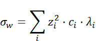
: Groundwater conductivity (S/m)

: Valence of ion

: Concentration of ion  (mol/m³)

: Ionic mobility (m²/Vs)

Higher groundwater conductivity leads to a stronger electrokinetic coupling and more pronounced seismo-electric signals. The seismo-electric effect is highly sensitive to variations in groundwater conductivity, making it a useful parameter in interpreting seismo-electric data (Revil & Jardani, 2013).

16. Groundwater Temperature

Groundwater temperature affects both the viscosity and the conductivity of the fluid, which in turn impacts the seismo-electric signals (Leroy & Revil, 2004). The temperature dependence of viscosity is described by the Arrhenius equation (Leroy & Revil, 2004):

· : Viscosity at temperature  (Pa·s)

· : Reference viscosity (Pa·s)

· : Activation energy (J/mol)

· : Universal gas constant (8.314 J/mol·K)

· : Temperature (K)

Changes in temperature can significantly alter the electrokinetic coupling, affecting the amplitude and frequency content of seismo-electric signals. Warmer groundwater generally leads to lower viscosity and higher conductivity, potentially enhancing the seismo-electric response (Revil & Jardani, 2013).

Geotechnical Parameters

17. Density

The density of a material is described as its mass per unit volume. Highly dense materials such as rock weigh more than less dense materials of similar volume such as gas or liquids. The mathematical description for density is shown in this equation.

ρ            = Density

m          = Mass of volume

V_s          = Total volume of solid mass

The density of a rock sample can be determined by measuring the dry mass of a sample material. This dry mass is attained by drying out the sample in an oven. The mass is then divided by the sample volume to obtain its density. A more accurate measure of the density of a porous consolidated rock is to measure its bulk density. The bulk density of a porous rock takes the average density of the grains of solid particles and the voids that make up the volume of the sample. Since sedimentary rock is formed by the consolidation of loose granules, the total volume consists of the void space between the consolidated granules as well as the volume of the solid granules themselves.  Equation 41 describes this. (Spitz & Moreno, 1996)

V_s          = Volume of the solids

V_v          = Volume of the voids

18. Porosity

Porosity is a measure of how much space or voids a porous material is made up of as a percentage or fraction of the material’s total volume. It is expressed as a fraction between 1 and 0 or 0% and 100% (Ramos da Silva, Schroeder, & Verbrugge, 2008). Porosity can be mathematically expressed as shown in this equation.

n            = Porosity

V_Voids     = Volume of voids

V_Total     = Total volume of material

There are a number of porosity types used to describe the porosity of an aquifer as a whole. This study assumes that the samples under test are very small in proportion to the dimensions of the aquifer they were extracted from. As such, they are assumed to be as homogeneous as possible.

19. Specific Volume

Specific volume is defined as the volume occupied by a specific mass of material. It is therefore the inverse of density. This equation shows this (Bueche, 1986).

W       = Density

m          = Mass of volume

V_s          = Total volume of solid mass

20. Shear Modulus

The shear modulus, also known as the modulus of rigidity, is defined as the ratio of shear stress applied to a material to the shear strain affected within it. Shear modulus is mathematically defined in this equation (Crandall & Dahl, 1959).

F / A     = shear stress

Δx / h   = shear strain

21. Bulk Modulus

Bulk modulus is a materials resistance to uniform compressional force. It is defined as the amount of pressure increase needed to affect a volume change on an object. This equation defines bulk modulus (Aster, 2006).

K            = Bulk modulus

V            = original volume

Δp         = Change in pressure

ΔV         = Change in volume

Bulk modulus can be categorized as either dry bulk modulus or wet bulk modulus. The dry bulk modulus is the modulus calculated for a sample that has no fluids present in its pore spaces between the grains of minerals that constitute the matrix. The wet bulk modulus is the modulus calculated for a sample where the pore spaces between the grains of minerals are saturated with fluids. The dry bulk modulus is donated by K_d, and the wet bulk modulus is notated by K_w. (Phani & Sanyal, 2008)

22. Young's Modulus

Young’s modulus describes the stiffness of a material and is known as the modulus of elasticity, elastic modulus or tensile modulus. It is the ratio of the rate of change between the stress applied, to the strain affected. (Hristopulos & Demertzi, 2008) This equation defines Young’s Modulus (Botha & Cloot, 2004):

E            = Young’s Modulus

σ            = Tensile Stress

ε            = Tensile Strain

Young’s modulus can also be used to determine the force exerted over a given area with a certain strain produced.

F            = Force exerted

E            = Young’s Modulus

A₀          = Area

ΔL         = Displacement

L₀           = Original length

23. Compressibility

Compressibility is the inverse of bulk modulus and is defined as the measure of volume change to applied pressure. It is defined by this equation (Fine & Millero, 1973).

K            = Bulk modulus

24. Lamé Constants

The Lame constants λ and μ can be calculated in a number of ways using a number of different elastic and physical rock properties. The Lame’s constants are material properties that are related to the elastic modulus and Poisson ratio. They define the stress to strain relations of a rock sample. The second Lame’s constant (u) is identical to the shear modulus (G). (Akiyoshi, Sun, & Fuchida, 1998)The equations below show these equations. (Weisstein, 2007)

E            = Young's modulus

v            = the Poisson ratio

G           = the shear modulus, K is the bulk modulus

p            = the density

Vp         = Compressional wave speed

Vs         = Shear wave speed

25. Poisson's Ratio

When an object is put under tensile stress, i.e. if it is stretched, it becomes longer and thinner. Poisson’s ratio is a measure of this as it measures the ratio of contractional strain to extensional strain. (Nieves, Gascon, & Bayon, 2007) The Poisson ratio can be described in terms of the Lamé constants λ and u as well as elastic parameters K and G and velocity values V_s and V_p.

          = Lame constant

u            = lame constant

K            = is the bulk modulus

U           = is the rigidity

Vp         = is the P-wave speed

Vs         = is the S-wave speed

26. Acoustic Impedance

The acoustic impedance of a material is the resistance to displacement of its particles by sound and occurs in many equations. Acoustic impedance is calculated as follows:

Z            = Acoustic Impedance

V_p          = Material Sound Velocity

ρ            = Material Density

The boundary between two materials of different acoustic impedances is called an acoustic interface. When sound strikes an acoustic interface at normal incidence, a part of the sound energy is reflected and a part is transmitted across the boundary (Wayne, Hykes, & Hedrick, 2005). The dB loss of energy, which is a logarithmic unit of measurement that expresses the magnitude of measurement relative to a referenced level of magnitude, on transmitting a signal from medium 1 into medium 2 is given by:

Z1         = Acoustic Impedance of First Material

Z2         = Acoustic Impedance of Second Material

The dB loss of energy of the echo signal in medium 1 reflecting from an interface boundary with medium 2 is given by (Wayne, Hykes, & Hedrick, 2005):

27. Clay Content

Clay content in a formation is often expressed as a percentage and can significantly affect the formation's electrical properties due to its cation exchange capacity (Revil & Jardani, 2013):

: Cation exchange capacity (cmol/kg)

High clay content increases the electrokinetic coupling due to the high surface area and cation exchange capacity, which can enhance seismo-electric signals, particularly in clay-rich formations (Revil & Jardani, 2013).

28. Frenzel Radius

The Frenzel radius () is defined as the radius within which the energy of a seismic wave is concentrated around the source. While not a standard equation, it is often conceptually related to the wavelength () of the seismic wave (Pride, 1994):

: Frenzel radius (m)

: Wavelength of the seismic wave (m)

The Frenzel radius influences the spatial resolution of seismo-electric surveys. Smaller Frenzel radii lead to higher resolution, enabling better detection of small-scale subsurface features (Pride, 1994).

29. Standard Penetration Test Number (SPTN)

The Standard Penetration Test Number (SPTN) is an empirical measure of soil resistance, defined by the number of hammer blows required to drive a sampler 30 cm into the soil. The relationship between SPTN and soil properties is given by (Sheriff & Geldart, 1995):

: Corrected SPT value (dimensionless)

: Recorded SPT value (dimensionless)

: Correction factor for hammer energy (dimensionless)

: Correction factor for borehole diameter (dimensionless)

: Correction factor for rod length (dimensionless)

: Correction factor for sampler (dimensionless)

SPTN can be correlated with the mechanical properties of the soil, such as density and shear strength, which are relevant for seismo-electric signal generation (Butler & Russell, 2003).

SPTN	Soil Packing	Relative Density
<4	Very Loose	<20
4-10	Loose	20-40
10-30	Compact	40-60
30-50	Dense	60-80
>50	Very Dense	>80

30. Rock Quality Designation (RQD)

Rock Quality Designation (RQD) is a measure of the quality of a rock mass based on the percentage of intact core pieces longer than 10 cm recovered during a core drilling process. It is calculated as (Deere, 1964):

RQD : Rock Quality Designation (percentage)

: Sum of lengths of core pieces longer than 10 cm (m)

: Length of the core run (m)

RQD provides an indication of rock mass quality, which affects the mechanical properties and fracture density of the rock. High RQD values generally correlate with higher mechanical strength and lower fracture density, which can influence the propagation and characteristics of seismo-electric signals (Butler & Russell, 2003).

RQD	Rock mass quality
<25%	very poor
25-50%	poor
50-75%	fair
75-90%	good
90-100%	excellent

Micro fracturing

Micro fractures are small cracks that appear in rock grains due to stress conditions. Micro fracturing occurs within rock grains for a number of reasons. The most common of these are sudden change in stress applied to a sample and mechanical stress placed on a sample volume by drilling extraction equipment such as core drills. (Sayers, 2007)

Micro fracturing affects acoustic pulse velocities in a rock sample in that it effectively slows the pulse down. When pressure is applied to a sample, these micro fractures are compressed closed and the acoustic velocity increases. As this pressure increases, the acoustic velocity increases until it becomes a linear increase of velocity. (Sayers, 2007). In the event that there is no micro fracturing, the compressional wave velocity is V_o. As pressure placed on the sample increases, so does the P-Wave velocity. This velocity increase is linear as long as the sample obeys Hooke’s law and stays within its linear elastic range. If micro fracturing is present the sample P-wave velocity will be lower by V_dif. As the pressure on the sample increases so does the p-wave velocity. This velocity increase is non-linear until the point is reached at P₁₀₀ where the micro factures are closed. The velocity increase is then linear from that point onwards. These velocity changes are typically very small. This study assumes that the velocity difference is smaller than the velocity error produced by the sampling rate and is thus ignored.

This equation relates these variable. (Přikryl, Lokajíček, Pros, & Klíma, 2007)

V_p          = Compressional wave velocity

V₀          = Velocity if no micro fracturing present

K_v          = Velocity coefficient

P            = Applied pressure

V_dif         = Difference in ideal and real velocity at atmospheric pressure

P_o          = Pressure at ideal velocities

31. Fracture Flow

Fracturing in the subsurface, particularly in rocks, plays a crucial role in fluid flow and can be characterized by fracture density, orientation, and aperture. The flow through fractures is often described by the cubic law (Bear, 1972):

: Volumetric flow rate (m³/s)

: Fracture aperture (m)

: Pressure difference across the fracture (Pa)

: Fluid viscosity (Pa·s)

: Length of the fracture (m)

Fracturing affects fluid flow paths, which can influence the generation and propagation of seismo-electric signals. Fractures with larger apertures and higher connectivity typically enhance fluid movement, leading to stronger seismo-electric responses (Revil & Jardani, 2013).

32. Compressional Velocity

Compressional velocity is a vector for rate of change of position. It is a measure of displacement over time in a given direction. If a longitudinal force is applied to an object, for instance, the end of solid cylinder, the longitudinal strains induced in the cylinder will travel down the cylinder away from the source. This Longitudinal displacement will move at a speed dictated by the elastic parameters of the cylinder. To calculate the longitudinal displacement velocity this equation can be applied. (Song & Suh, 2004)

V_c          = The compressional velocity

Δx         = Distance traveled

Δt          = Time passed to travel distance

The longitudinal velocity of a material can be determined by its bulk modulus, shear modulus and density. This equation defines this relation. (Song & Suh, 2004)

K =        Bulk modulus

V_p =      Compressional wave velocity

G =       Shear modulus

 =        Density of the rock sample

33. Shear velocity

Shear velocity is a vector for rate of change of position. It is a measure of displacement over time in a given direction. If a shear force is applied to an object, for instance, the end of solid cylinder, the shear strains induced in the cylinder will travel down the cylinder away from the source. This shear displacement will move at a speed dictated by the elastic parameters of the cylinder. To calculate the shear displacement velocity this equation can be applied. (Song & Suh, 2004)

V_s          = the shear velocity

Δx         = Distance traveled

Δt          = Time passed to travel distance

The shear velocity of a material can be determined by its shear modulus and density. This equation defines this relation. (Song & Suh, 2004)

G =       Shear modulus

V_s =       Shear velocity

 =        Density of the rock sample

Interpretations

Artificial intelligence algorithms are employed to interpret the geohydrological and geotechnical data in order to estimate lithology and aquifer type and condition.

34. Interpreted Lithology (Formation Type)

This data set describes the interpreted lithology of the formations under the site. It is derived from the estimated geotechnical properties calculated for the formations under the site and referenced against averaged rock properties gathered from multiple global lithological studies to interpret which major lithological group a formation may be assigned to. The interpreted lithology descriptor and description for the lithological groups available are shown below.

Lithology Description	Lithology Descriptor
Soil	1-      SL
Unconsolidated Sediment	2-      US
Volcanics	3-      VO
Conglomerates	4-      CO
Consolidated Sediments	5-      CS
Igneous	6-      IG
Salt	7-      ST
Mafic	8-      MA
Metamorphic	9-      ME
Ultra Mafic	10- UM

35. Condition

This data set describes the condition of the formations under the site. It is derived from the estimated geotechnical properties calculated for the formations under the site and referenced against averaged rock properties gathered from multiple global lithological studies to interpret the condition a formation may be in. The formation conditions and description are shown below.

Condition	Condition Descriptor
Soil	1
Fine grained	2
Course grained	3

Fractured	4-6-8-10-12-14
Porous	5
Weathered	5-7-9-11-13-15
Unaltered	16

36. Interpreted Aquifer Classification (Aquifer Type)

This data set describes the interpreted aquifer classifications for the formations detected under the sounding location. The aquifer classification is defined by the geo-hydrological and lithological properties of the formations under the sounding location. The interpreted aquifer classification descriptor and description for the aquifer classification groups available are shown below.

Aquifer Classification Description	Aquifer Classification Descriptor
Ultra-Mafic Rock Aquifer	1-      UM
Fractured Ultra Mafic Rock Aquifer	2-      FU
Metamorphic Rock Aquifer	3-      MP
Fractured Metamorphic Rock Aquifer	4-      FP
Weathered Mafic Rock Aquifer	5-      WM
Fractured Mafic Rock Aquifer	6-      FM
Weathered Igneous Rock Aquifer	7-      WI
Fractured Igneous Rock Aquifer	8-      FI
Conglomerate Aquifer	9-      CA
Fractured Conglomerate Aquifer	10- FC
Volcanic Rock Aquifer	11- VA
Fracture Volcanic Rock Aquifer	12- FV
Sedimentary Rock Aquifer	13- SR
Fractured Sedimentary Rock Aquifer	14- FS
Unconsolidated Dual Porosity Sedimentary Aquifer	15- DP
Unconsolidated Sedimentary Aquifer	16- SA
Saturated Soil Aquifer	17- SS

37. Aquifer Types

Aquifers are classified based on their hydraulic properties, such as confined, unconfined, and perched aquifers. These classifications affect how water is stored and transmitted within the subsurface (Bear, 1972). The type of aquifer influences the seismo-electric response. For example, confined aquifers tend to generate more pronounced seismo-electric signals due to the higher pressure buildup compared to unconfined aquifers, where the pressure is more evenly distributed (Revil & Jardani, 2013).

Different Types of Aquifers Detectable by Seismo-Electric Data

Seismo-electric data can be used to detect and characterize different types of aquifers based on the interaction between seismic waves and the subsurface’ s fluid content. Aquifers are generally classified into several types, each with distinct characteristics that influence their seismo-electric responses.

Unconfined Aquifers

Definition: Unconfined aquifers are those where the water table is open to the atmosphere through the pore spaces of the overlying material. The water level in a well penetrating an unconfined aquifer corresponds to the water table (Bear, 1972).

Seismo-Electric Response:

· Characteristics: In unconfined aquifers, the seismo-electric signal is primarily influenced by the porosity and permeability of the material. The interaction between seismic waves and the freely moving groundwater results in a seismo-electric signal that can be used to map the water table and delineate the aquifer boundaries.

· Interpretation: AI models can be trained to recognize the characteristic patterns of unconfined aquifers, such as the slower rise time of the seismo-electric signal due to the gradual response of the water table to seismic waves (Revil & Jardani, 2013).

Confined Aquifers

Definition: Confined aquifers are bounded above and below by impermeable layers, known as aquitards, and the water within these aquifers is under pressure (Bear, 1972).

Seismo-Electric Response:

· Characteristics: Confined aquifers typically produce stronger seismo-electric signals due to the higher pressure gradients created by seismic waves. The presence of impermeable layers also affects the signal's amplitude and frequency content.

· Interpretation: AI techniques can help differentiate confined aquifers from unconfined ones by analyzing the pressure-induced variations in the seismo-electric response. Confined aquifers often show a quicker rise time and higher amplitude signals compared to unconfined aquifers (Revil & Jardani, 2013).

Perched Aquifers

Definition: Perched aquifers occur when an impermeable layer or lens traps water above the main water table, creating a localized zone of saturation (Bear, 1972).

Seismo-Electric Response:

· Characteristics: Perched aquifers typically produce localized seismo-electric signals. The presence of a perched water table can be identified by a distinct, often isolated, seismo-electric anomaly corresponding to the trapped water.

· Interpretation: AI models can be used to detect these localized anomalies, distinguishing them from broader aquifer systems. The AI approach can also assist in determining the extent and thickness of the perched aquifer by analyzing the spatial variation of the seismo-electric signals (Revil & Jardani, 2013).

Artesian Aquifers

Definition: Artesian aquifers are a type of confined aquifer where the pressure is sufficient to cause water to rise above the top of the aquifer in wells, and in some cases, even above the ground surface (Bear,

1972).

Seismo-Electric Response:

· Characteristics: The high-pressure conditions in artesian aquifers can lead to particularly strong seismo-electric responses. The pressure gradients created by seismic waves can cause rapid fluid movement, generating significant electrokinetic signals.

· Interpretation: The seismo-electric response from artesian aquifers can be distinguished by AI models trained to recognize the high amplitude and rapid rise time signals characteristic of such high-pressure systems (Revil & Jardani, 2013).

The integration of artificial intelligence into the interpretation of lithology using seismo-electric data represents a significant advancement in geophysical exploration. AI enables more accurate, efficient, and detailed analysis of complex seismo-electric datasets, improving the understanding of subsurface characteristics. Additionally, the ability of seismo-electric methods to detect and differentiate between various aquifer types—such as unconfined, confined, perched, and artesian aquifers—highlights the versatility and value of this approach in hydrogeological investigations.

Electric Parameters

38. Apparent Resistivity

Electrical resistivity (also called volume resistivity or specific electrical resistance) is a fundamental specific property of a material that measures its electrical resistance or how strongly it resists electric current. A low resistivity indicates a material that readily allows electric current. Resistivity is commonly represented by the Greek letter ρ (rho). The SI unit of electrical resistivity is the ohm-meter (Ω⋅m). Resistivity is defined by the following equation :

R – Resistance

ρ – Resistivity A – Area

L - length

GIS Parameters

The GIS data sets discussed in this section are derived from global GIS databases and describe general and averaged GIS metrics over the globe. These data sets are not intended to provide accurate hydrological and geological information about the investigation site but rather they provide generalized information of the areas around an investigation site. These data sets are not used in the evaluation or interpretation of the geophysical,geohydrological, geological or geotechnical data collected and discussed in this report, but rather provide context to the findings and recommendations discussed and made in this report. The GIS parameters provided are as follows:

39. Satellite Imagery

This data is useful in assessing the layout of the survey locations in relation to geographical features such as infrastructure, dams, rivers, coastlines, mountain ranges and the like. The map shows the locations of the surveyed points with point number labels. The recommended drilling locations are indicated by numbered label icons, numbered in the order of recommendation from recommendation one to recommendation nine, as illustrated in the Map Marker Legend. It is possible to show only the recommended drilling locations by selecting the “Show only recommendation points” checkbox, located in the Site map settings section, beneath the map. It is possible to download the map and corresponding survey point data, by selecting the “Download Map” option, located above the map. Additionally, the map shows the coordinates, in WGS84 Decimal degrees, of the mouse pointer hovering over the map, on the top right corner of the map. The map scale is indicated on the bottom right corner of the map.

When any of the survey points on the map are selected, a popup menu will appear, indicating the parameters of the selected point. This includes:

1. The point number

2. The point drilling recommendation index

3. The point Latitude and Longitude in WGS84 decimal degree format

4. The point elevation, in meters above sea level (masl) as recorded by the GPS system onboard the GeoVision hardware system.

5. The calculated sustainable yield estimate for the survey point in liters per second, for the depth range defined by the user on the GeoVision system when interpreting the project data.

6. The calculated maximum yield estimate for the survey point in liters per second, for the depth range defined by the user on the GeoVision system when interpreting the project data.

7. The calculated minimum yield estimate for the survey point in liters per second, for the depth range defined by the user on the GeoVision system when interpreting the project data.

8. The calculated static ground water level estimate for the survey point in meters below ground level (mbgl).

9. The interpreted recommended maximum drilling depth for the selected survey point location in meters below ground level (mbgl)

10. The calculated overall risk percentage associated with the selected point due to the site noise recorded at the point, the lithological setup under the point, the recorded data quality, correlation and the signal to noise ratio for the sounding location. This parameter defines the risk associated with the analysis and interpretation results of the data collected at the selected survey point.

11. The confidence level, as a percentage, in the analyzed and interpreted results for the selected survey point data. This parameter indicates the calculated level of confidence the GeoVision system has in the results for the selected point, with regard to the reported data and yield estimate calculations, with the risk parameter considered.

12. The correlation parameter indicates the correlation index, expressed as a percentage, between the individual data sets collected during the sounding. It is a measure of the quality of the collected data.

13. The signal to noise ratio (SNR) parameter indicates the amplitude ratio between the recorded noise and geophysical responses received. It is a measure of data quality for the selected survey point.

40. Lithology

This data is useful in assessing the layout of the survey locations in relation to surface lithology and can be used to determine the basic lithology a survey is conducted on. The map shows the locations of the surveyed points with point number labels. The recommended drilling locations are indicated by numbered label icons, numbered in the order of recommendation from recommendation one to recommendation nine. The map scale is indicated on the bottom right corner of the map.

41. Faulting

This data is useful in assessing the layout of the survey locations in relation to regional faulting structures under the survey area. The recommended drilling locations are indicated by numbered label icons, numbered in the order of recommendation from recommendation one to recommendation nine. The map scale is indicated on the bottom right corner of the map.

42. Water Shed

This data is useful in assessing the layout of the survey locations in relation to the water shed boundaries around the survey area. This data provides insight into the natural flow direction of groundwater around the survey area. The recommended drilling locations are indicated by numbered label icons, numbered in the order of recommendation from recommendation one to recommendation nine. The map scale is indicated on the bottom right corner of the map.

43. Regional Aquifer Classification

This data is useful in assessing the layout of the survey locations in relation to the known aquifers around the survey area. This data provides insight into the possible quality of aquifer in the area surrounding the survey area. The recommended drilling locations are indicated by numbered label icons, numbered in the order of recommendation from recommendation one to recommendation nine. The map scale is indicated on the bottom right corner of the map.

44. Static Groundwater Level

This data is useful in assessing the layout of the survey locations in relation to the static groundwater levels around the survey area. This data provides insight into the depth the static water table may be encountered around the survey area. The recommended drilling locations are indicated by numbered label icons, numbered in the order of recommendation from recommendation one to recommendation nine. The map scale is indicated on the bottom right corner of the map.

45. Saline Aquifers

This data provides insight into the possibility of saline aquifers in the area around the survey area. The recommended drilling locations are indicated by numbered label icons, numbered in the order of recommendation from recommendation one to recommendation nine. The map scale is indicated on the bottom right corner of the map.

46. Geothermal Resources

This data provides insight into the geothermal resources under the survey area and as such provides insight into the geothermal potential in the area surrounding the survey site and whether the survey area has potential for geothermal formations or is on a known geothermal field. The recommended drilling locations are indicated by numbered label icons, numbered in the order of recommendation from recommendation one to recommendation nine. The map scale is indicated on the bottom right corner of the map.

Additional Information

47. Point Data Traces

To view the graphical representation of all the data collected for a specified point in the project, as one-dimensional data trace, use the Point Data Traces Feature. Simply select the point for which the data is to be shown from the dropdown list.

48. Point Virtual Logs

To view the virtual well log, containing all data regarding a specified project point, use the Point Virtual Logs feature. Simply select the point for which the virtual log data is to be shown from the dropdown list.To download the log to an excel file, select the Export to Excel button located at the bottom of the log.

 49. Report Views

All the interactive data plots provide the user functions to create both local plot and general presentation views, that can be save and viewed at a later time.

50. Local Views

Local views allow the user to save and reload plot views created by the user for each individual plot on the report. The term local view is used as the saved plots apply only to the chart they were created in, as such they can only be reloaded into the same plot they were created in. Loading views do not require that the plot be regenerated, as such the load times are much faster than if the plot was regenerated. A maximum of 20 local views can be created for each plot chart in the report. This is done by first generating the plot in the configuration of choice. The user then selects the view the plot views is to be saved to from the dropdown list under the Create Site Section Line Views, Create site Profile Views or the Create Site Model Views subsections, located under every plot. The user then enters a description for the view and then selects the Save view option. The view is now saved. To load the view, simply select the view from the same dropdown list and select the Load View button. The view will be loaded.

 It is important to note that the view is not saved to a local file on the PC but stored in the computer’s volatile memory. As such if the document is closed, the views created will be lost unless saved to a file on the PC.

51. General Presentation Views

General Presentation views allow the user to save and reload plot views created by the user in any plot of the report, then view them on the Presentation view plot, located at the end of the report. The term general presentation view is used as the saved plots apply to any plot in the report, however, they can only be viewed in the Presentation View plot located at the end of the report. This is done to allow the user to build a presentation of custom views from any plot in the report and view them in one plot, the presentation views plot. Loading views do not require that the plot be regenerated, as such the load times are much faster than if the plot was regenerated. A maximum of 20 local views can be created for each plot chart in the report. This is done by first generating the plot in the configuration of choice. The user then selects the view the plot views is to be saved to from the dropdown list under the Create Presentation Views subsections, located under every plot. The user then enters a description for the view and then selects the Save view option. The view is now saved. To load the view, simply scroll down to the Presentation view plot, located at the end of the document, and select the view from the dropdown list then select the Load View button. The view will be loaded in the presentation view plot.

It is important to note that the view is not saved to a local file on the PC but stored in the computer’s volatile memory. As such if the document is closed, the views created will be lost unless saved to a file on the PC. This is discussed later.

52. Saving Views to a local PC folder

To save all local and general presentation views created for the report to a file located within a local folder on the host PC, use the Save All View Data to File option located under the View Controls section at the end of the report. This will save and download the views to the local downloads folder of your device. The report can now be closed, and the views reloaded at a later time.

53. Loading Views from a local PC folder

To reload the views saved to a file on the local host PC, simply use the Load all View Data from File, function located under the View Controls section at the end of the report. This will allow the user to select the previously save view file on the host PC and reload the view data into the report.

References

Books and Book Chapters:

• Bear, J. (1972). Dynamics of Fluids in Porous Media. Elsevier.
• Breiman, L. (2001). Random Forests. Machine Learning, 45(1), 5-32.
• Cortes, C., & Vapnik, V. (1995). Support-vector Networks. Machine Learning, 20(3), 273-297.
• Hinton, G. E., & Salakhutdinov, R. R. (2006). Reducing the Dimensionality of Data with Neural Networks. Science, 313(5786), 504-507.
• Jolliffe, I. T. (2002). Principal Component Analysis (2nd ed.). Springer.
• LeCun, Y., Bengio, Y., & Hinton, G. (2015). Deep Learning. Nature, 521(7553), 436-444.
• Sheriff, R. E., & Geldart, L. P. (1995). Exploration Seismology (2nd ed.). Cambridge University Press.
• Spitz, K., & Moreno, J. (1996). A Practical Guide to Groundwater and Solute Transport Modeling. John Wiley and Sons.
• Ugural, A., & Fenster, S. (2003). Advanced Strength and Applied Elasticity. Prentice Hall.

Journal Articles:

• Akiyoshi, T., Sun, X., & Fuchida, K. (1998). General absorbing boundary conditions for dynamic analysis of fluid-saturated porous media. Soil Dynamics and Earthquake Engineering, 17, 397–406.
• Argatov, I., & Sabina, F. (2008). Acoustic diffraction by a finite number of small soft bodies. Wave Motion, 45, 238–253.
• Biot, M. A. (1956). Theory of propagation of elastic waves in a fluid-saturated porous solid. Journal of the Acoustical Society of America, 28(2), 168-191.
• Biot, M. A. (1962). Generalized theory of acoustic propagation in porous dissipative media. Journal of the Acoustical Society of America.
• Botha, J. F., & Cloot, A. H. (2004). Deformations and the Karoo aquifers of South Africa. Advances in Water Resources, 27(4), 383–398.
• Butler, K. E., & Russell, R. D. (2003). The seismoelectric method: Theory and application. Surveys in Geophysics, 24(1), 47-81.
• Deere, D. U. (1964). Technical description of rock cores for engineering purposes. Rock Mechanics and Engineering Geology, 1(1), 16-22.
• Fine, R., & Millero, F. (1973). Compressibility of water as a function of temperature and pressure. Journal of Chemical Physics, 59, 10.
• Gang, H., & Maurice, B. (2003). Description of fluid flow around a wellbore with stress-dependent porosity and permeability. Journal of Petroleum Science and Engineering, 40, 1 – 16.
• Gercek, H. (2007). Poisson’s ratio values for rocks. International Journal of Rock Mechanics and Mining Sciences, 44(1), 1-13.
• Hristopulos, D., & Demertzi, M. (2008). A semi-analytical equation for the Young’s modulus of isotropic ceramic materials. Journal of the European Ceramic Society, 28, 1111–1120.
• Jennings, D., & Flint, A. (1995). Introduction to Medical Electronics Applications. Butterworth-Heinemann.
• Knudby, C., & Carrera, J. (2006). On the use of apparent hydraulic diffusivity as an indicator of connectivity. Journal of Hydrology, 377– 389.
• Komodromos, P. (2007). Simulation of the earthquake-induced pounding of seismically isolated buildings. Computers and Structures, 1-9.
• Leroy, P., & Revil, A. (2004). A triple-layer model of the surface electrochemical properties of clay minerals. Journal of Colloid and Interface Science, 270(2), 371-380.
• Madeira, M. M., Bellis, S. J., & Beltran, L. A. (1999). High-performance computing for real-time spectral estimation. Control Engineering Practice, 7(5), 679-686.
• Mikhailov, O., Queen, J., & Toksoz, M. N. (2000). Using borehole electroseismic measurements to detect and characterize fractured (permeable) zones. Geophysics, 65(4), 1098-1112.
• Nieves, F., Gascon, F., & Bayon, A. (2007). An analytical, numerical, and experimental study of the axisymmetric vibrations of a short cylinder. Journal of Sound and Vibration.
• Phani, K., & Sanyal, D. (2008). The Relations between the Shear Modulus, the Bulk Modulus and Young’s Modulus for Porous Isotropic Ceramic Materials. Materials Science and Engineering A.
• Pride, S. R. (1994). Governing equations for the coupled electromagnetics and acoustics of porous media. Physical Review B, 50(21), 15678-15696.
• Sayers, C. M. (2007). Effects of borehole stress concentration on elastic wave velocities in sandstones. International Journal of Rock Mechanics and Mining Sciences, 44(7), 1045-1052.
• Song, I., & Suh, M. (2004). Determination of the elastic modulus set of foliated rocks from ultrasonic velocity measurements. Engineering Geology, 72, 293–308.
• Wang, Y. C., & Lakes, R. S. (2003). Lakes Resonant ultrasound spectroscopy in shear mode. Review of Scientific Instruments, 74(3), 1371-1373.
• Zadler, B., Jerome, H. L., & Le Rousseau, J. (2004). Resonant Ultrasound Spectroscopy: Theory and Application. Geophysical Journal International, 156(1), 154-169.
• Zhu, Z., & Toksoz, M. N. (2003). Cross-well seismoelectric measurements in boreholes. Geophysics, 68(5), 1519-1524.